Request the desired data in the most suitable format from the Abaqus.
The major consideration is the required accuracy of data.
The major constraint is what is available in your Abaqus solver.
For example, Abaqus/Explicit does not have the capability to write
output data in a human readable form in the data file.
If the demands for accuracy are modest, and if you are
using Abaqus/Standard, and if the
variable you want can be written to the data file
(.dat),
and most of them can be,
then requesting the output to the
data file
is the easiest.
For this you use commands such as
*NODE PRINT,
*EL PRINT,
etc. in the input,
(.inp) file:
*NODE PRINT,FREQUENCY=100,TOTALS=NO,SUMMARY=NO
COORD,U1,U2
that might give you something like this
for a 2D model in the data file, (.dat):
   THE FOLLOWING TABLE IS PRINTED FOR ALL NODES

       NODE FOOT-   COOR1       COOR2       U1          U2
            NOTE

          3       100.0      -19.00       0.000       0.000
          4       50.00       17.50       0.000      -5.751
          5       125.0       12.50      -1.449       2.925
          6       124.0       12.50      -1.449       2.809
          7       123.0       12.50      -1.449       2.694
          8       122.0       12.50      -1.449       2.578
          9       121.0       12.50      -1.449       2.462
         10       120.0       12.50      -1.449       2.346
         11       119.0       12.50      -1.449       2.230
         12       118.0       12.50      -1.449       2.114
         13       117.0       12.50      -1.449       1.998
         14       116.0       12.50      -1.449       1.882
As you can see, the accuracy is only to 4 significant digits. AFAIK, it is not possible to increase the accuracy of the data written in the data file. If you know better, let me know.
So imagine I have two steps in the analysis, and what I want
to know is the change in some variable between
the steps.
In principle I can dump the variable from both steps to the
.dat
file and then subtract
one from the other for all points.
However, if the accuracy of the data is poor, the subtraction
is likely to loose the useful data completely.
Here's a relaxation example. I need to know displacement difference between 2 steps. The displacements themselves are:
                        S T E P       4     S T A T I C   A N A L Y S I S
                                INCREMENT     9 SUMMARY
   THE FOLLOWING TABLE IS PRINTED FOR ALL NODES

       NODE FOOT-   COOR1       COOR2       U1          U2
            NOTE

          3       100.0      -19.00       0.000       0.000
          4       50.00       17.50       0.000      -5.751
          5       125.0       12.50      -1.449       2.925
          6       124.0       12.50      -1.449       2.809
          7       123.0       12.50      -1.449       2.693
          8       122.0       12.50      -1.449       2.577
          9       121.0       12.50      -1.449       2.461
         10       120.0       12.50      -1.449       2.345
                        S T E P       5     S T A T I C   A N A L Y S I S
                                INCREMENT     1 SUMMARY
   THE FOLLOWING TABLE IS PRINTED FOR ALL NODES

       NODE FOOT-   COOR1       COOR2       U1          U2
            NOTE

          3       100.0      -19.00       0.000       0.000
          4       50.00       17.50       0.000      -5.751
          5       125.0       12.50      -1.449       2.925
          6       124.0       12.50      -1.449       2.809
          7       123.0       12.50      -1.449       2.694
          8       122.0       12.50      -1.449       2.578
          9       121.0       12.50      -1.449       2.462
         10       120.0       12.50      -1.449       2.346
So when you calculate the difference, you get fuck all:
node     coord1  coord2	     delta u1        delta u2

3        100.00  -19.00      0.0000          0.0000
4         50.00   17.50      0.0000          0.0000
5        125.00   12.50      0.0000          0.0000
6        124.00   12.50      0.0000          0.0000
7        123.00   12.50      0.0000          0.0010
8        122.00   12.50      0.0000          0.0010
9        121.00   12.50      0.0000          0.0010
10       120.00   12.50      0.0000          0.0010
In other words, there is no useful data left at all.
So, if you use the explicit dynamic solver (Abaqus/Explicit),
where output to
.dat
file is not available,
or if the accuracy is not good enough, the print output is no good.
The solution is to use results file.
Requesting output to the
results file
is easy.
Note that on Abaqus/Standard this is
.fil
file,
and on Abaqus/Explicit this is the
selected results file,
.sel file, which can later be
converted to
.fil format.
The beauty is that virtually anything can be written
to the results file, and in the raw solution accuracy,
i.e. typically with 6 or 16 significant digits for single
and double precisions respectively.
You use
*EL FILE,
*NODE FILE
and so on, e.g.:
*NODE FILE,FREQUENCY=100
COORD,U
However, getting the data out of
.fil
files is hard.
The
.fil
file is binary, consists of variable length records
in a fucked up archaic Abaqus format.
You have to write your own fortran code to do this.
The
manual
does help a lot though.
First study the format of the results file. Understanding it it critical. I'll just give a summary here, that is necessary for understanding the rest. As the manual says, each record consists of N 8-byte long words. The first word in the record gives the record length. This is not very useful. The second word is the "record type key". This is a of critical importance. This is simply an integer numerical label uniquely identifying the type of data in the following words, so that you know how to interpret it. All words starting from third and until the end of the record contain the actual data that you might want. The manual calls these "attributes".
For example, the key for nodal displacement is 101:
Record key: 101           Output variable identifier: U
Record type: Displacements
Attributes:  1 - Node number.
             2 - First component of displacement.
             3 - Second component of displacement.
             4 - Etc.
Note that you need to shift attribute numbers by 2 to get the correct word from the record. So the 1st attribute is in word 3, the 2nd attribute is in word 4, etc.
A major complication arises due to the
fact that integer, real and character data
are all written in 8-byte words.
Correctly reading them requires some tricks.
Again,
the manual
helps.
There is a complete working example in the manual.
Also, here is my
routine
to read the displacement and coordinate data,
written with
*NODE FILE above.
For completeness, and if you want to check that all works as
I claim it does, use this routine with this
input file.
So, as the manual says,
you have to make sure to read integer and real
variables into integer and real arrays respectively,
which are linked by the
EQUIVALENCE statement.
The EQUIVALENCE statement
is deprecated in Fortran 1995 and later standards.
Deprecated means the use of this language feature
is discouraged, but it's still supported by
the standard.
If you've never used it,
there are lots of on-line references, e.g.
for
Oracle,
VMS
or
Intel
Fortran compilers.
So, using
EQUIVALENCE
the code might look like this:
 dimension  array(513), jrray(nprecd,513), lrunit(2,1)
 equivalence (array(1), jrray(1,1))

 if ( key .eq. 1901 ) write (101,*) jrray(1,3), array(4:5)
Here
jrray is integer, but array is real.
Both contain words from a single record in the results file.
You use Abaqus make to build the executable of your routine, like this:
abaqus make -j filread.f
This will create the executable, in this
case filread.exe.
Now you run it:
abaqus filread
and get your data out,
exactly as you wrote in your filread.f.
In my case I send the displacement and the coordinate data
in two separate files.
I got my files, say coord
with nodal coordinates and
disp with displacements:
bigblue3> head disp
Step  4 increment   9
           3  0.000000000000000E+000  0.000000000000000E+000
           4  1.428079566719941E-045  -5.75109246300800
           5  -1.44881443711145        2.92463968914136
           6  -1.44881444100420        2.80876287022771
           7  -1.44881447839977        2.69288604816396
           8  -1.44881455541383        2.57700916562378
           9  -1.44881465370697        2.46113216774218
          10  -1.44881474476933        2.34525500817265
          11  -1.44881479233482        2.22937764679067
bigblue3> head coord
           3   100.000000000000       -19.0000000000000
           4   50.0000000000000        17.5000000000000
           5   125.000000000000        12.5000000000000
           6   124.000000000000        12.5000000000000
           7   123.000000000000        12.5000000000000
           8   122.000000000000        12.5000000000000
           9   121.000000000000        12.5000000000000
          10   120.000000000000        12.5000000000000
          11   119.000000000000        12.5000000000000
          12   118.000000000000        12.5000000000000
bigblue3>
Note that I now have 16 significant digits in my data.
A bit of manual work is requred now.
I send the step and increment data to the displacement file,
so that it contains displacements for two stages in the
analysis.
I split
disp into
disp1 that contains displacements
at stage 1 and
disp2 that contains displacements
at stage 2:
bigblue3> wc disp*
  19358   58076 1180760 disp
   9676   29028  590236 disp1
   9676   29028  590236 disp2
  38710  116132 2361232 total
bigblue3>
and remove all other verbal info, I leave just the numerical data.
The next step is automatic.
I make a single file out of
disp1,
disp2 and
coord,
by combining the rows for the same nodes.
I remove unused columns and sort the data
in numerical order, first by column 2,
then by column 1.
The following step is very important. Both PGPLOT and gnuplot work best when the data is on a rectangular grid, i.e. there is a constant spacing between all data points along x1, and a constant, but possibly different, spacing between all data points along x2. This is a severe limitation on the mesh used for the analysis. Although you can use some interpolation package and create a rectilinear data from some arbitrary mapping, it is easiest, of course, to use a mesh of rectangular 1st order elements. In this example, we used 2nd order elements, so the easiest way is to remove all rows (or all columns) with intermediate nodes.
Finally, to make the most of gnuplot the data must consist of blocks, which are data lines with the same x1 or x2. The blocks are separated by a single blank line, i.e. a line containing only the newline or carrier return symbol.
I use awk for all these data manupulation tasks. I put the awk commands into a makefile.
So I have two files:
data, which I'll use with
PGPLOT:
bigblue3> head data
3280 0.000000000000000E+000 -12.5000000000000 0.000274330783040 0.000687236486760
9680 0.500000000000000 -12.5000000000000
3279 1.00000000000000 -12.5000000000000 0.000266323464180 0.000695243805620
9678 1.50000000000000 -12.5000000000000 -0.013380064313444 0.007915329657459
3278 2.00000000000000 -12.5000000000000 -0.014548465230992 0.009710210354360
9676 2.50000000000000 -12.5000000000000 -0.011055213069521 0.004830879022210
3277 3.00000000000000 -12.5000000000000 -0.012213001424994 0.006280364714549
9674 3.50000000000000 -12.5000000000000 -0.008848870617161 0.002485569495919
3276 4.00000000000000 -12.5000000000000 -0.009927510401962 0.003568737254870
9672 4.50000000000000 -12.5000000000000 -0.006872776989411 0.000806080620250
bigblue3>
and
data.grid, which differs from
data only by having extra blank
line every time the third column, x2
coordinate changes.
I'll use data.grid with
gnuplot.
Here's the PGPLOT program I use to draw contour plots. It is adapted from the PGPLOT demo programs. I use this Makefile to build it.
The key routine is
PGCONT.
There is a little bit of manual work involved.
In particular, you have to specify the spacing
between the data points, and the origin,
which is the TR input to the
PGCONT routine.
And you need to calculate the number of data points
along x1 and x2,
which determines the size of the array F.
The second key routine is PGCONL, which applies labels to the contous.
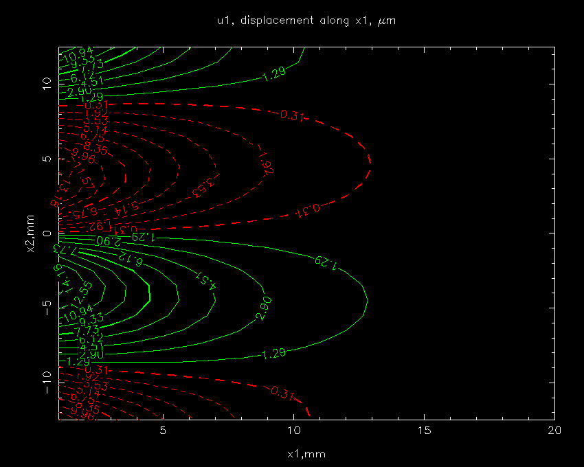
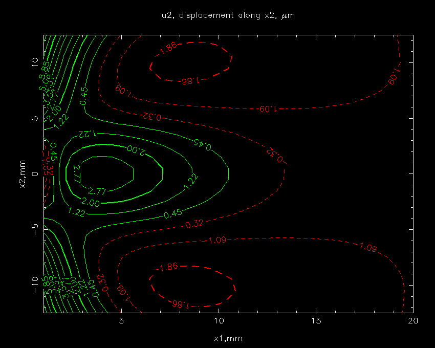
And here's the result. Green solid lines are positive. Red dashed lines are negative:
For gnuplot I use this script. It is a lot simpler than the PGPLOT program, but the results are not as good:


Apparently it is possible to add labels to contour lines, but I haven't tried that. These links (thanks to Graeme Horne) give the details:
http://gnuplot-tricks.blogspot.co.uk/2009/07/maps-contour-plots-with-labels.html